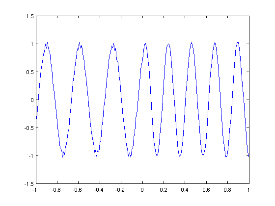
function [ ] = hwk2()

% Set time and space step sizes
h = 0.01;
lambda = 0.5;
k = h*lambda;

% Set wave speeds
a1 = 1;
a2 = 0.7;

% Set initial values
M = 2/0.01;             % Number of intervals in x-axis
x = -1:h:1;             % x_0, x_1, x_2, ... x_M
u = zeros(M+1, 1);      % initial condition
uold = u;               % uold will store the value from previous time step

% Prepare figure, clear figure, and set axis ranges
figure(1);
clf;
axis([-1 1 -1.5 1.5]);

% Time step t_1, calculated using forward-time backward-space
t = k;                  % Current time variable value
u(1) = sin(20*t);       % Since at t=0, the initial condition is identically 0,
                        % there isn't much to compute and hence we only
                        % need to set the left boundary.
% Draw the graph and prepare for making the movie.
plot(x,u);
axis([-1 1 -1.5 1.5]);
F(1) = getframe;

% Time steps t_2, t_3, ...
% In order to get enough frames to make a nice movie, we will compute 600
% time steps, that is from t_2 to t_{601}
for n=1:600
    t = (n+1)*k;        % Current time variable value
    uoldold = uold;     % For leap-frog, we need to store two previous time steps
    uold = u;
    u(1) = sin(20*t);   % Set left boundary

    % For x<=0, use wave speed a1 = 1
    u(2:101) = uoldold(2:101) - a1*lambda*(uold(3:102)-uold(1:100));
    % For x>0, use wave speed a2 = 0.7
    u(102:200) = uoldold(102:200) - a2*lambda*(uold(103:201)-uold(101:199));

    % Set right boundary
    u(201) = 2*uold(200) - uoldold(199);

    % Plot solution for every 10 time steps and prepare for movie.
    if mod(n,10)==0
        plot(x,u);
        axis([-1 1 -1.5 1.5]);
        F(n/10+1) = getframe;
    end
end

% Make the movie
movie(F,1)

end

Published with MATLAB® 7.13