prog2demo

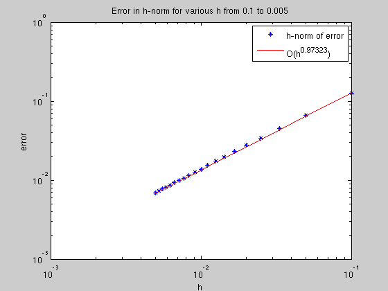
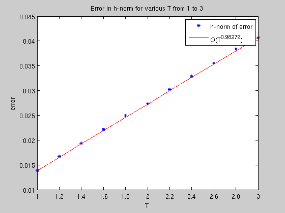
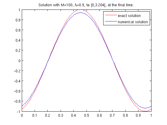
function prog2demo
  % lambda should be set as strictly less than 1 here
  lambda = 0.9;
  % plotdata = 0 forbids upwindscheme to plot solutions
  plotdata = 0;

  % In the first experiment, we fix lambda, t0, tN, and compare the h-norm of
  % the error at the final time step for various space step size h
  M = 10:10:200;
  error = zeros(size(M));
  for i=1:length(M)
    [h,x,uexact,unumerical] = upwindscheme(M(i),lambda,0,1,plotdata);
    error(i) = hnorm(h,uexact,unumerical);
  end
  r = linearlinefitting(1./M, error);  % compute the order k of error = O(h^k)
  figure(10);
  clf;
  loglog(1./M, error, '*', 1./M, error(1)*(M(1)./M).^r ,'r');
  xlabel('h');
  ylabel('error');
  legend('h-norm of error',['O(h^{' num2str(r) '})'])
  title(['Error in h-norm for various h from ' num2str(1/M(1)) ' to ' num2str(1/M(end))]);

  % In the second experiment, we fix M, lambda, t0 and compare the h-norm of the
  % error at the final time step for various final time T = tN
  % We know the error = C_T O(h^k) when the solution is smooth enough.
  % For fixed h, we would like to check how C_T depends on T.
  t = 1:0.2:3;
  error = zeros(size(t));
  for i=1:length(t)
    [h,x,uexact,unumerical] = upwindscheme(100,lambda,0,t(i),plotdata);
    error(i) = hnorm(h,uexact,unumerical);
  end
  r = linearlinefitting(t, error);
  figure(20);
  clf;
  plot(t, error, '*', t, error(1)*t.^r ,'r');
  xlabel('T');
  ylabel('error');
  legend('h-norm of error',['O(T^{' num2str(r) '})'])
  title(['Error in h-norm for various T from ' num2str(t(1)) ' to ' num2str(t(end))]);

  % plot the solution for M=100, lambda=0.9, at final time step 3.2
  upwindscheme(100,0.9,0,3.2,1);

%%%%%%%%%%%%%%%%%%%%%%%%%%%%%%%%%%%%%%%%%%%%%%%%%%%%%
% this function computes || u-v ||_h norm
function [err] = hnorm(h,u,v)
  err = sqrt(h) * norm(u-v,2);

%%%%%%%%%%%%%%%%%%%%%%%%%%%%%%%%%%%%%%%%%%%%%%%%%%%%%
% Given a sequence of row vectors x, y=O(x^r)
% This function computes the order k by using linear fitting.
function [r] = linearlinefitting(x,y)
  x = log(x);
  y = log(y);
  r = (length(x)*(x*y') - sum(x)*sum(y))./(length(x)*sum(x.^2)-(sum(x))^2);

%%%%%%%%%%%%%%%%%%%%%%%%%%%%%%%%%%%%%%%%%%%%%%%%%%%%%%%%%%%%%%%%%%%%%%%%%%%%
%%------------------------------------------------------------------------%%
 %   Solve the one-way wave equation using 1st order upwind scheme        %
 %                                                                        %
 %     u_t + u_x = 0      for 0<x<1, 0<t<T                                %
 %                                                                        %
 %     with periodic boundary condition u(0) = u(1)                       %
 %                                                                        %
 %   Function arguments are:                                              %
 %     M  -- number of intervals in space direction                       %
 %     lambda  --  k/h                                                    %
 %     [t0,tN] --  time range                                             %
 %                 if tN/k is not an integer, we reset tN such that       %
 %                 it is the closest number that gives an integer tN/k    %
 %     plotdata -- if plotdata>0, then the solution is ploted             %
 %                 in the figure window No. plotdata                      %
 %                                                                        %
 %     h -- returns space step size                                       %
 %     x -- returns linspace(0,1,M+1)                                     %
 %     uexact -- exact solution at time tN on x coordinates given by x    %
 %     uN -- numerical solution at time tN                                %
%%------------------------------------------------------------------------%%

function [h,x,uexact,u] = upwindscheme(M,lambda,t0,tN,plotdata)
  h = 1.0/M;
  k = h*lambda;
  N = round((tN-t0)/k);
  tN = k*N;

  % set initial condition
  x = linspace(0,1,M+1);
  u = initialcondition(x);

  % For time step 1 to N, calculate u using the previous time step data.
  for n=1:N
    u = u-lambda * [u(1)-u(M),diff(u)];
  end

  % exact solution at tN
  shiftedx = x-tN;
  uexact = initialcondition(shiftedx - floor(shiftedx));

  % plot solution
  if (plotdata)
    figure(plotdata);
    clf;
    plot(x,uexact,'r',x,u,'b');
    legend('exact solution', 'numerical solution');
    title(['Solution with M=' num2str(M) ', \lambda=' num2str(lambda) ', t\in [' ...
	num2str(t0) ',' num2str(tN) '], at the final time.']);
  end

%%%%%%%%%%%%%%%%%%%%%%%%%%%%%
% Given vector x= (x0, x1, ... xM), compute the initial data
function [v0]=initialcondition(x)
  v0 = sin(2*pi*x);
  %v0 = double(x>0.25&x<=0.75);