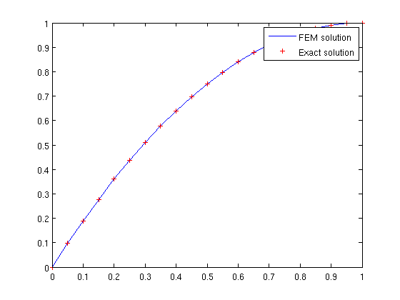
function fem1dlinear
% This function solves the 1D BVP
%  -au'' + bu' + cu = f     in (x0, x1)
% with either Dirichlet or Neumann boundary conditions at x0 and x1.
%
% The problem is solved using a finite element method
% using the continuous piecewise linear approximation space.
%

%
% Variables
% =========================================
% coefficients: a structure containing three coefficients a,b,c in the equation.
%               They are stored in coefficients.a, coefficients.b, coefficients.c
%
% leftbdr, rightbdr: Two structures defining the boundary conditions on x0 and x1.
%                    Each contains three components, we use leftbdr as an example:
%                      leftbdr.x = x0
%                      leftbdr.type is either 'Dirichlet' or 'Neumann'
%                      leftbdr.value: for Dirichlet boundary condition, it is
%                                     the value of u(x0); for Neumann boundary
%                                     condition, it is the value of u'(x0)
%                    The definition of rightbdr is similar.
%
% f: the right-hand function. It is defined using "function handle".
%    See matlab help for more about function handle.
%
% n: number of sub-intervals.
%
% x: A row vector containing the x-coordinates of all grid nodes.
%    It needs to be monotonically increasing, and x(1) = x0, x(end) = x1.
%
% A, rhs, u: the linear system derived from the finite element approximation is
%               A u = rhs
%
%
% Subroutines
% =========================================
% assembleLocalMatrix
% assembleLocalRhs
%


% =====================================================================
% PART I:  initialization
% =====================================================================
% In this part, we set up the problem.
% You can change the settings here in order to solve a different problem.

  % setting coefficients
  coefficients.a = 1;
  coefficients.b = 5;
  coefficients.c = 5;

  % set left boundary condition
  leftbdr.x = 0;
  leftbdr.type = 'Dirichlet';
  leftbdr.value = 0;

  % set right boundary condition
  rightbdr.x = 1;
  rightbdr.type = 'Neumann';
  rightbdr.value = 0;

  % set right-hand side function f
  f = @(x) 12-5*x.*x;

  % set number of intervals and generate grid
  % For now, a uniform grid is generated.
  % One can rewrite this part to generate a non-uniform grid.
  n = 20;
  x = linspace(leftbdr.x, rightbdr.x, n+1);


% =====================================================================
% PART II:  finite element discretization
% =====================================================================
% In this part, we assemble the linear system using the finite element method.
% Then solve the linear system.

  % assemble matrix A
  A = sparse(n+1,n+1);
  for i=1:n % on each sub-interval [x(i), x(i+1)]
    localmat = assembleLocalMatrix(x(i),x(i+1),coefficients);
    A(i:i+1,i:i+1) = A(i:i+1,i:i+1) + localmat;
  end

  % assemble right-hand side vector rhs = (f,v)
  rhs = zeros(n+1,1);
  for i=1:n % on each sub-interval [x(i), x(i+1)]
    localrhs = assembleLocalRhs(x(i),x(i+1),f);
    rhs(i:i+1) = rhs(i:i+1) + localrhs;
  end

  % apply left boundary condition
  if strcmp(leftbdr.type, 'Dirichlet')
    % make the first row (1,0,0,...,0), and set rhs(1)
    A(1,:) = 0;
    A(1,1) = 1.0;
    rhs(1) = leftbdr.value;
    % change 2:end entries of rhs,
    % then erase 2:end entries in the first column of A
    rhs(2:end) = rhs(2:end) - A(2:end,1) * leftbdr.value;
    A(2:end,1) = 0;
  else % Neumann bdr condition
    rhs(1) = rhs(1) - coefficients.a * leftbdr.value;
  end

  % apply right boundary condition
  if strcmp(rightbdr.type, 'Dirichlet')
    % make the last row (0,...,0,0,1), and set rhs(end)
    A(end,:) = 0;
    A(end,end) = 1.0;
    rhs(end) = rightbdr.value;
    % change 1:end-1 entries of rhs,
    % then erase 1:end-1 entries in the last column of A
    rhs(1:end-1) = rhs(1:end-1) - A(1:end-1,end) * rightbdr.value;
    A(1:end-1,end) = 0;
  else % Neumann bdr condition
    rhs(end) = rhs(end) + coefficients.a * rightbdr.value;
  end

  % solve
  u = A \ rhs;


% =====================================================================
% PART III:  print out the result
% =====================================================================

  % for the current problem, we know that its exact solution is
  %   u = x(1-x)
  plot(x, u, 'b', x, x.*(2-x), 'r+');
  legend('FEM solution', 'Exact solution');

%%%%%%%%%%%%%%%%%%%%%%%%%%%%%%%%%%%%%%%%%
% This is the end of the main function. %
%%%%%%%%%%%%%%%%%%%%%%%%%%%%%%%%%%%%%%%%%


% =====================================================================
% PART IV:  subroutines
% =====================================================================
% This part contains some sub-functions.

%%%%%%%%%%%%%%%%%%%%%%%%%%%%%%%%%%%%%%%%%%%%%%%%%%%
% This is to compute (au',v') + (bu',v) + (cu,v)
% on the subinterval [a,b]
function localA = assembleLocalMatrix(a,b,coefficients)
  h = b-a;
  localA = coefficients.a / h * [1, -1; -1, 1] ...
      + coefficients.b * [-0.5, 0.5; -0.5, 0.5] ...
      + coefficients.c * h * [1/3, 1/6; 1/6, 1/3];

%%%%%%%%%%%%%%%%%%%%%%%%%%%%%%%%%%%%%%%%%%%%%%%%%%%
% This is to compute (f,v) on the subinterval [a,b].
% A Gaussian quadrature will be used to evaluate the
% integral. Here we use a 5th order scheme. You can
% change "5" into what ever order you would like to use.
function localrhs = assembleLocalRhs(a,b,f)
  % First, compute the Gaussian points and weights.
  % Both gaussianpoints and gaussianweights are column vectors.
  [gaussianpoints, gaussianweights] = lgwt(5,a,b);

  % evaluate the value f on Gaussian points
  % fvalue is a column vector
  fvalue = f(gaussianpoints);

  % evaluate the value of two basis functions
  %    (b-x)/(b-a)  and   (x-a)/(b-a)
  % on gaussianpoints.
  % "shape" is a matrix with two columns, each column
  % contains the value of one basis function on gaussianpoints.
  h = b-a;
  shape = [ (b-gaussianpoints)/h, (gaussianpoints-a)/h ];

  % apply the gaussian quadrature to compute localrhs
  localrhs = shape' * (fvalue.*gaussianweights);