function [] = dispersion()

% (1) Illustration of the dispersion effect

M = 500;
N = 100;
x = linspace(0,10, M+1);

figure(1); clf;
F(N) = struct('cdata',[],'colormap',[]);
for n=1:N
    t = n*0.1;
    u = cos(x-t) + 0.1*cos(20*(x-t));
    plot(x, u);
    title('No dispersion');
    drawnow;
    F(n) = getframe;
end
movie(F);

figure(2); clf;
F(N) = struct('cdata',[],'colormap',[]);
for n=1:N
    t = n*0.1;
    u = cos(x-t) + 0.1*cos(20*(x-2*t));
    plot(x, u);
    title('Dispersion');
    drawnow;
    F(n) = getframe;
end
movie(F);


% (2) Dispersion in numerical scheme
M = 200;
x = linspace(0,10, M+1);
N = 200;
h = 10/200;
a = 1;
lambda = 0.6;
k = lambda*h;

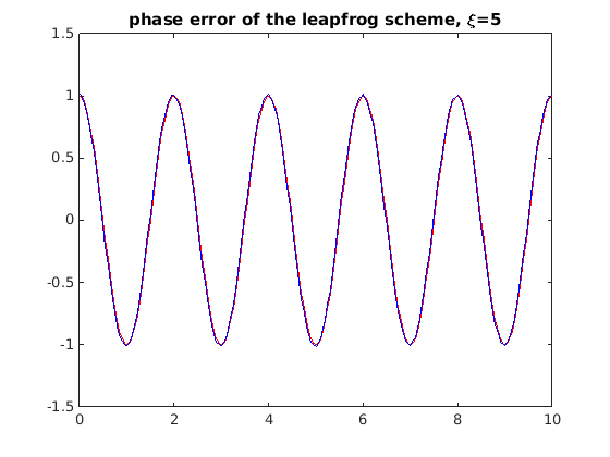
xi = 5;
u0 = cos(xi*pi/5*x);
u = LeapFrog (M, N, u0, lambda);
t = N*k;
figure(3); clf;
plot(x, cos(xi*pi/5*(x-a*t)), 'r', x, u(N+1,:),'b');
title('phase error of the leapfrog scheme, \xi=5');


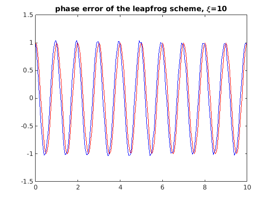
xi = 10;
u0 = cos(xi*pi/5*x);
u = LeapFrog (M, N, u0, lambda);
t = N*k;
figure(4); clf;
plot(x, cos(xi*pi/5*(x-a*t)), 'r', x, u(N+1,:),'b');
title('phase error of the leapfrog scheme, \xi=10');

end


function [u] = LeapFrog(M, N, u0, lambda)
% Implementation of the leap frog scheme
u = zeros(N+1, M+1);
u(1,:) = u0;
% Use forward-time central space to compute the solution at t_1
% period boundary condition
u(2, 2:M) = u(1,2:M) - 0.5*lambda*u(1,3:(M+1)) + 0.5*lambda*u(1,1:(M-1));
u(2,1) = u(1,1) - 0.5*lambda*u(1,2) + 0.5*lambda*u(1,M);
u(2,M+1) = u(2,1);
% The leap frog scheme starts from t_2
for n=3:(N+1)
    u(n, 2:M) = u(n-2,2:M) - lambda*( u(n-1,3:(M+1)) - u(n-1,1:(M-1)) );
    u(n,1) = u(n-1,1) - 0.5*lambda*u(n-1,2) + 0.5*lambda*u(n-1,M);
    u(n,M+1) = u(n,1);
end
end

Published with MATLAB® R2014b