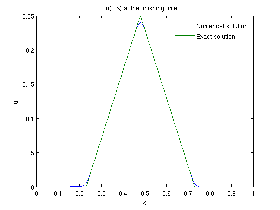
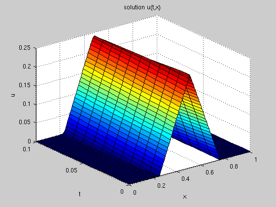
%%------------------------------------------------------------------------%%
 %   Solve the one-way wave equation                                      %
 %                                                                        %
 %     u_t + a u_x = 0      for 0<x<1, 0<t<T                              %
 %                                                                        %
 %              | 0   for 0<x<0.25                                        %
 %     u(0,x) = | x-0.25   for 0.25<x<0.5    the initial condition        %
 %              | 0.75-x   for 0.5<x<0.75                                 %
 %              | 0   for 0.75<x<1                                        %
 %                                                                        %
 %     u(t,0) = 0   if a>0                  the boundary condition        %
 %     u(t,1) = 0   if a<0                                                %
 %                                                                        %
 %   In this example, we only use forward space-discretization.           %
 %                                                                        %
 %   In the beginning, you can set the following values:                  %
 %      a  -- wave speed                                                  %
 %      M  -- number of space intervals                                   %
 %      k  -- time step size                                              %
 %      N  -- number of time steps (the final time T = k*N)               %
 %      time_discretization = 'forward' or 'backward'                     %
%%------------------------------------------------------------------------%%

% First, we need to set some parameters ...
a = -0.2;
M = 100;
k = 1.0/M;
N = 10;
time_discretization = 'forward';
%time_discretization = 'backward';

% set h and lambda = k/h.
% DO NOT change them manually, they should be calculated
h = 1.0/M;
lambda = k/h;


% Now, let's solve the problem using the finite difference method

% generate a (N+1)-by-(M+1) matrix to store data
u = zeros(N+1,M+1);

% set the initial condition
x = linspace(0, 1, M+1);     % generate a (M+1)-dim vector x
for m=1:M+1
  if x(m) <= 0.25
    u(1,m) = 0.0;
  elseif x(m) <= 0.5
    u(1,m) = x(m)-0.25;
  elseif x(m) <= 0.75
    u(1,m) = 0.75-x(m);
  else
    u(1,m) = 0.0;
  end
end %for i

% For time step 2 to N, calculate u using the previous time step data.
% This process is different for forward/backward time schemes.
if isequal(time_discretization,'forward')   % forward time
  for n=2:N+1
    for m=1:M
      u(n,m) = u(n-1,m) - a*lambda*( u(n-1,m+1) - u(n-1,m) );
    end
    % now set the boundary condition
    if a<0
      u(n,M+1) = 0.0;
    else
      u(n,M+1) = u(n,M);   % in downwind scheme, manually set outflow boundary
    end
  end % for t
elseif isequal(time_discretization,'backward')   % backward time
  for n=2:N+1
    % for backward scheme (implicit), we need to solve
    % a linear system in each time step.
    % First, set the linear system ...
    A = sparse(M+1,M+1);       % A is an (M+1)*(M+1) sparse matrix
    f = zeros(M+1, 1);         % f is an (M+1)-dim vector
    for m=1:M
      A(m,m) = 1-a*lambda;
      A(m,m+1) = a*lambda;
      f(m) = u(n-1,m);
    end
    % now set the boundary condition
    if a<0 % set the last equation u(n,M+1) = 0
      A(M+1, M+1) = 1;
      f(M+1) = 0;
    else  % set the last equation u(n,M+1)-u(n,M) = 0
      A(M+1,M+1) = 1;
      A(M+1, M) = -1;
      f(M+1) = 0;
    end
    % solve the linear system for u(t+1,:), A\f computes A^{-1} f
    % a single quote will do a tranpose,
    %   which makes the column vector (A\f) into a row vector
    u(n,:) = (A\f)';
  end %for t
end %if time_discretization


% Next, we should view the results...
% print the settings on screen
T = N*k;
fprintf('The settings are: \n');
fprintf('    k = %f,    h = %f,   lambda = %f \n',k,h,lambda);
fprintf('    After %d time steps, we end at T = %f \n\n', N, T);
% draw the solution at t=T
% we know the exact solution at t=T is u_0(x-aT)
x_minus_at = linspace(0,1,M+1) - a*T;
exactsol = zeros(1,M+1);
for m=1:M+1
  if x_minus_at(m) <= 0.25
    exactsol(1,m) = 0.0;
  elseif x_minus_at(m) <= 0.5
    exactsol(1,m) = x_minus_at(m)-0.25;
  elseif x_minus_at(m) <= 0.75
    exactsol(1,m) = 0.75-x_minus_at(m);
  else
    exactsol(1,m) = 0.0;
  end
end %for i
figure(1); clf;
plot(x,u(N+1,:),x,exactsol);
legend('Numerical solution','Exact solution');
title('u(T,x) at the finishing time T');
xlabel('x'); ylabel('u');
% draw the suface u(t,x)
[x,t] = meshgrid(0:h:1,0:k:(k*N));
figure(2); clf;
surf(x,t,u);
title('solution u(t,x)');
xlabel('x'); ylabel('t'); zlabel('u');

The settings are: 
    k = 0.010000,    h = 0.010000,   lambda = 1.000000 
    After 10 time steps, we end at T = 0.100000 

Published with MATLAB® 7.6