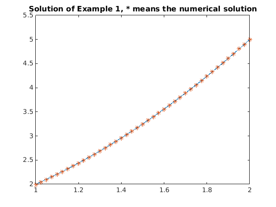
f = @(t,y) (2*y-2)/t;
[t,y] = ode45(f, [1, 2], 2);
figure(1); clf;
plot(t,t.^2+1);
hold on
plot(t,y,'*');
hold off
title('Solution of Example 1, * means the numerical solution');
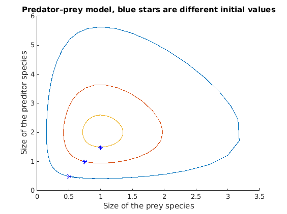
f = @(t,x) [4*x(1)-2*x(1)*x(2); -3*x(2)+3*x(1)*x(2)];
figure(2); clf;
hold on
[t,x] = ode45(f, [0, 2.2], [0.5,0.5]);
plot(x(:,1), x(:,2));
[t,x] = ode45(f, [0, 2.2], [0.75,1]);
plot(x(:,1), x(:,2));
[t,x] = ode45(f, [0, 2.2], [1,1.5]);
plot(x(:,1), x(:,2));
plot([0.5, 0.75, 1], [0.5, 1, 1.5], 'b*');
hold off
title('Predator–prey model, blue stars are different initial values');
xlabel('Size of the prey species');
ylabel('Size of the preditor species');
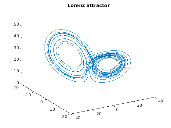
f = @(t,x) [-10*x(1)+10*x(2); 28*x(1)-x(2)-x(1)*x(3); -8/3*x(3)+x(1)*x(2)];
[t,x] = ode45(f, [0, 20], [-8,8,27]);
figure(3); clf;
plot3(x(:,1), x(:,2), x(:,3));
title('Lorenz attractor');
view(60,30);