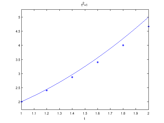
N = 5;
figure(1);
clf;
ezplot('t^2+1',[1,2]);
hold on;
h = 1/N;
t = 1;
w = 2;
plot(t,w,'*');
for i=1:N
w = w + h*(2*w-2)/t;
t = 1 + i*h;
plot(t,w,'*');
end
error = (2^2+1) - w;
fprintf('When h = %2.2f, the error at t=2 is %5.4f\n',h, error);
hold off
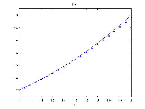
N = 10;
figure(2);
clf;
ezplot('t^2+1',[1,2]);
hold on;
h = 1/N;
t = 1;
w = 2;
plot(t,w,'*');
for i=1:N
w = w + h*(2*w-2)/t;
t = 1 + i*h;
plot(t,w,'*');
end
error = (2^2+1) - w;
fprintf('When h = %2.2f, the error at t=2 is %5.4f\n',h, error);
hold off;
N = 20;
figure(3);
clf;
ezplot('t^2+1',[1,2]);
hold on;
h = 1/N;
t = 1;
w = 2;
plot(t,w,'*');
for i=1:N
w = w + h*(2*w-2)/t;
t = 1 + i*h;
plot(t,w,'*');
end
error = (2^2+1) - w;
fprintf('When h = %2.2f, the error at t=2 is %5.4f\n',h, error);
hold off;
When h = 0.20, the error at t=2 is 0.3333
When h = 0.10, the error at t=2 is 0.1818
When h = 0.05, the error at t=2 is 0.0952