NewtonsDivDiff2

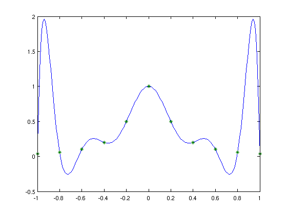
% Use Newton's forward difference to interpolate
% function f(x) at n+1 points.
%
% Pay attention that the indices in Matlab
% start from 1, while it starts from 0 in the algorithm
% given in class. You need to shift the indices in the program.

% Set n, x_i and f(x_i)
n = 10;
x = [-1 -0.8 -0.6 -0.4 -0.2 0 0.2 0.4 0.6 0.8 1];
fx = [0.0385 0.0588 0.1 0.2 0.5 1 0.5 0.2 0.1 0.0588 0.0385];

% The values f(x_i) are stored in the first column of
% an (n+1)*(n+1) matrix F.
F = zeros(n+1, n+1);
F(:, 1) = fx;

% Compute the Newton divided differences.
for i=1:n
    for j=1:i
        F(i+1,j+1) = (F(i+1,j)-F(i,j)) / (x(i+1)-x(i-j+1));
    end
end

% Print out the coefficients of the interpolation,
% which is given by F(1,1), F(2,2), F(3,3), ... F(n+1,n+1).
% Then the Lagrange interpolation is
% (here all indices have been shifted so it starts from 1 and end at n+1)
%  F(1,1) + F(2,2)*(x-x1) + F(3,3)*(x-x1)*(x-x2) + ...
%         + F(n+1,n+1)*(x-x1)*(x-x2) ... (x-xn)
% We can use the Matlab command "diag" to get these diagonal elements.
a = diag(F)

% Next, we would like to draw the graph of the Lagrange interpolation.
% To do this, we first need to evaluate the polynomial at a set of points.
% The x and y coordinates of these points are stored in plotx and ploty.
plotx = -1:0.01:1;
% Evaluate the value of the Lagrange interpolation "Horner-style".
ploty = a(n+1)*ones(size(plotx));
for i=n:(-1):1
    ploty = a(i) + ploty.*(plotx-x(i));
end

% Draw the graph.
% The curve is the interpolation,
% and the given points (x_i, f(x_i)) are shown as stars.
figure(1);
plot(plotx, ploty, '-', x, fx, '*');